Lab 7 - March 18, 2015 - Modeling Friction Forces

Lab 7:

March 18, 2015

Brandon Elder

Modeling Friction Forces

Purpose: This lab is split into five parts. The purpose of the first two parts is to use a system of masses, string, wooden blocks, force sensor, and a pulley to determine the coefficients of static and kinetic friction. The purpose of the third and forth part of the lab is to measure the angle at which a block slides down a ramp and measure a mass of a block and use this information to determine the coefficients of friction, some static and some kinematic. The last part's purpose is to use one of the coefficients of kinetic friction we determined to then predict the acceleration of a two-mass system.

Part 1: Measuring Static Friction

Set up the apparatus to look like Fig. 1. Measure the block before you begin. We measured a mass of 131 grams. 

Fig. 1 The apparatus includes a wooden block, with felt, connected by a string to a cup with
water. The cup was filled with water slowly until the block began to move. The amount of water
that was added to the cup is the amount of force that was required to make the system move.

The following steps were taken for the rest of the process.

• Gradually fill the foam cup, the one suspended in the system, with water until the block(s) resting on the table, begin moving. This point represents the value for the max. static friction. Stop adding water the very instant that the block begins to move. 
• Weigh the mass of the cup, with the water still in it. 
• Stack another block on top of the block which is tied to End A of the string. 
• Repeat all previous steps. 

We repeated the experiment, adding one block to the system with each repeat until we had four blocks stacked. The data that we recorded is below, in Fig. 2. The free body diagram of the system is shown below in Fig. 2 as well.

Fig. 2 The recorded values of our block weights and the cup weight when filled with enough water to make the system move. This experiment was performed four times.

Even though we used LoggerPro to determine the coefficient of static friction, we also performed all calculations in order to double check (See Fig 2a and 2b).

Fig. 2a Calculations for the coefficient of static friction. The free body diagram and sum
of forces equations are all drawn on this paper.

Fig 2b The remaining calculations for the 3rd and 4th block trials. The average coefficient
was determined here as well.

Fig. 3 Data inputted into LoggerPro.

In order to graph this data to determine the coefficient of the maximum static friction, we needed to input this data into LoggerPro (See Fig. 3). The slope of the graph of the friction force and the normal force data gives up our coefficient of static friction. In this case, our coefficient of static friction was .305 (See Fig. 4).

Fig. 4 Slope of the line on the graph determines our coefficient of friction static in this experiment.

Part 2: Kinetic Friction

Fig. 5 Force sensor attached to wooden block and pulling it
 across the table at a constant velocity.

Next, we determined the coefficient of kinetic friction. We accomplished this by attaching a force sensor to a string to a block. We then pulled the block across a table at a constant velocity (no acceleration). (See Fig. 5). LoggerPro measure the force that was required to pull the block across the table. Fig. 6 shows the data inputted into LoggerPro and the graphs of the data. From this graph we can determine the average force required to pull each block across the table at a constant speed. We then took that data and made a new data table and graphed the data. From that table, (See Fig. 6a) we were able to look at the slope of the best fit line, which is the coefficient of the kinetic energy.

Fig. 6 These four graphs represent the four trials performed with the four blocks with the force sensor. 

Fig. 6 These four graphs represent the four trials performed with the four blocks with the force sensor. 

Fig. 6a All four pulls are graphed here and the slope of the line is the coefficient of friction - kinetic.

Part 3: Static Friction from a Sloped Surface.

The purpose of this part is to measure the coefficient of static friction, once again. Except this time, we will be using an inclined ramp to track the block. The process is simple. We placed a block with a felt bottom on a board and slowly raised the board until the block started to slide down. Once the block slid down we measured the angle at which the board was at (See Fig. 7 and 8).

Fig. 7 The angle is being measured of the ramp. The block slid down the ramp at this angle.

Fig. 8 The block sliding down the ramp.

The angle at which the block begins to slide is the angle we will use for theta in our sum of forces calculations. Start by drawing out a free body diagram of the set up. The sum of forces in the x-direction (parallel to the ramp) are going to be mg(sin(theta)) = the static friction, because we are looking for the amount of f(static) there is no acceleration to take into account for.  The angle we measured was 19.8 degrees and the mass of the block was 122 grams. With these two pieces of information we were able to perform the calculations (See Fig. 9) and determine the coefficient of static friction to be 0.36. Funny thing is that the coefficient ended up being just the tangent of theta... LOL

Fig. 9 The sum of forces calculations and free body diagram used to determine the coefficient of static friction.

Part 4: Kinetic Friction from Sliding a Block Down an Incline

The purpose of this portion of the lab is to determine the coefficient of kinetic friction of the block as it slides. Because we know that it takes more force to get something to move than to keep it in motion, we are expecting that this coefficient of kinetic friction will be less that what we discovered in part 3 above. The way we will determine the friction is by using a motion detector to track the acceleration of the block as it slides down. We will also record the angle at which the ramp is placed while the block slides down. Once we have those two pieces of information we can set up our free body diagrams and our sum of forces equations (See Fig. 10). The coefficient of kinetic friction for this experiment was 0.337, which is in line with our assumption from above. The kinetic friction force is less than the static friction force.

Fig. 10 The free body diagrams and the sum of forces equations and calculations.

Part 5: Predicting the Acceleration of a Two-Mass System

In this final part of the lab we will take the coefficient of kinetic friction from above, .337, and use it to determine an equation for the acceleration of a block being pulled across a table in a two-mass system exactly like the set-up of part 1 (See Fig. 1). The mass hanging from the string must be big enough to move the system (because we are using the kinetic friction). We will then measure the acceleration in LoggerPro and compare the measured acceleration to our calculated acceleration. The diagrams, formulas, and calculations are below (See Fig. 11). We determined the acceleration on the system to be -.087 m/s2. When we plugged in the motion detector to LoggerPro to measure the acceleration of the block as it slid across the table, the value for acceleration that we received was 0.9458, which is very close.

Fig. 11 The formulas used and diagrams used to estimate what the acceleration on the system would be. 

Conclusion:

We started by using the block-water pulley system to find the coefficient of static friction between the block and the table and graphing the force of static friction with the normal force of the block to find a relationship. The relationship was the coefficient of static friction.

Then we used the force sensor to calculate the kinetic friction of the experiment using the force graph of the recorded data. After that we found the coefficient of static friction of the wooden block on top of an inclined ramp. Next, we used the acceleration found from the block sliding down a steep ramp with the motion sensor to calculate the coefficient of static friction for the ramp. Finally we predicted the acceleration of the system by using the previous coefficient of static friction.

Lab 6 - March 11, 2015 - Propagated Uncertainty in Measurements

Lab 6:
Brandon Elder
3/11/2015

Propagated Uncertainty in Measurements

Purpose: To learn how to calculate the propagated error in each of our density measurements of three pieces of metal. An additional purpose is to calculate the mass of two unknown objects hanging from spring scales and to determine the propagated uncertainty in the calculated value of the mass.

Fig. 1 Calipers used to measure the length and diameter
of all three masses.

Gathering Data: Obtain a pair of calipers (see Fig. 1) a box of masses. Choose three of the masses and measure the height and diameter of all three. Put together the weights with the measurements in a table (see Fig. 2). After all the measurements are taken, weigh the objects on a scale to get the mass.

Fig. 2 Graph of three different masses. Aluminum, Copper,
and Lead.

Fig. 3 Formula for the
volume of a cylinder.

Fig. 4 Formula used to calculate
density. (D=M/V)

Calculations: 

Volume: First, calculate the volume for all three objects. Volume of a cylinder is: (pi * radius squared * height) (see Fig. 3). All calculations were recorded on our white board (see Fig. 2).

Density: The formula for calculating density is (mass / volume) (see Fig. 4).

Fig. 5 Known uncertainties in measurements. the uncertainty
in these calipers is .1 mm because the measurement will
always be between .1 mm increments. 

 Ok, that was the easy part. Now we have a table of data that has some numbers on it. But we must ask ourselves, how certain are we that these numbers are accurate? Anytime that a measurement is taken there will be some degree of uncertainty. For example, when we take a measurement, the object being measured will most likely fall between two divisions on our scale. The reading will come down to a judgement call on the user's end about which division the object is closer to and this is the uncertainty that is always present in any measurement (see Fig. 5). These uncertainties are called known uncertainties. It is a combination of known uncertainties in measurements that leads to unknown uncertainty in the final result.

Fig. 6 In the top of the picture we see the formula used to calculate density.
Underneath it we see the formula that will be used to calculate "dp" the
uncertainty in density.

Propagated Uncertainty: Propagate means to spread out. When we spread out known uncertainties we create unknown uncertainty. Uncertainty in density calculations comes from three different calculations, the mass, diameter, and the height calculations. We must create an equation for density that we can use to calculate the amount of uncertainty in our density measurement. We know that we have three uncertainties, m, l, and h. We also know that density = m/v. We need an equation that has all of our uncertainties in it. If we substitute the formula used to calculate the volume, we will have density = m/(pi*(d/2)^2*h. This simplifies to (4/pi)*(m/(d^2*h) (See Fig. 6).

Take the derivative of the function for each different variable, m, d, and h, respectively. Then, plug the numbers into the new equations and this will give you the "dp/dm", "dp/dd", and "dp/dh" portions of the equation (middle of Fig. 6). The formulas used to calculate these are in Fig. 7.

Fig. 7 Formulas used from the partial derivatives.

The known uncertainty in mass, diameter, and height are taken form the devices used to measure the numbers. The mass is .1 grams, the diameter is .1 cm, and the height is .01 cm (See Fig. 7a). See Fig. 8 and Fig. 9 for the calculations of all three object's unknown, propagated uncertainties. As you can see from our measurements, the calculated densities plus the propagated uncertainties are all within the ranges of the known values of their densities.

Fig. 7a Entire calculation with all formulas for propagated uncertainties.

Fig. 8 Aluminum and Copper Density with uncertainties.

Fig. 9 Lead's density with propagated uncertainty calculated.

Determination of an Unknown Mass:

Next, we are going to apply our knowledge of uncertainty to an unknown mass hanging from a pair of spring scales (see Fig. 10). We will need to measure the angles and record the spring scale readings (see Fig. 11). Then, we used the measured values to determine the mass of the unknowns. The formula used to determine the mass is written down in Fig 11a. The partial derivatives were taken (See Fig. 12) to calculate the propagated error for each variable: F1, F2, theta1 and theta2. Fig. 13 and 14 has the calculations completed for both unknown masses and the amount of uncertain error.

Fig. 11a Formula used to calculate mass is located to the
right of the diagram.

Fig. 10 Unknown mass hanging from
two spring scales.

Fig. 11 Measured angles and
Spring Scale readings.

Fig. 12 Partial derivatives.

Fig. 13 Unknown mass #2 with
propagated uncertainty formula.

Fig. 14 Unknown mass #1 with
propagated uncertainty.

Lab 3 - March 7, 2015 - Non-Constant Acceleration Problem/Activity with EXCEL

Lab 3:
Brandon Elder
March 7, 2015

Non-Constant Acceleration Problem/Activity with EXCEL

Purpose: To find how far an elephant on roller skates will travel, with a rocket (strapped to his back) firing above his head in the opposite direction, before he his direction changes (See Fig. 1). We will investigate these distance questions analytically (physics) and numerically (Excel).

Fig. 1 How far will the rocket let the elephant travel
before he changes direction?

Problem: A 5000-kg elephant on frictionless roller skates is going 25 m/s when it gets to the bottom of a fill and arrives on level ground. At that point a rocket mounted on the elephant's back generates a constant 8000 N thrust opposite the elephant's direction of motion. The mass of the rocket changes with time (due to burning the fuel at a rate of 20 kg/s) so that the: 

m(t) = 1500 kg - 20 kg/s*t.

Find how far the elephant goes before coming to rest.

Fig. 2 Acceleration as a function of time.

Fig. 3 Finding the change in velocity in order to
derive an equation for v(t).

Fig. 4 At the bottom of the picture you will see the equation
for x(t). Thanks to the professor!

Fig. 5 The result of plugging the time into the postion
equation. Result: 248.7 meters.

Analytically: We were given the acceleration of the elephant plus the rocket as a function of time (See Fig. 2). From the acceleration function we can integrate from 0 to t to find the change in velocity and then to derive an equation for v(t) (See Fig. 3). Following the same logic, we can integrate the velocity function from 0 to t to find the change in X and then use this to derive an equation for x(t) (See Fig. 4). Next, we find the time at which the velocity is zero. As this will be the time we can plug into the distance formula to solve for the length the elephant travels before turning around. Plugging in the result of 19.69075 seconds results in a distance of 248.7 meters (See Fig. 5). Next, we will analyze the same problem numerically by using Excel.

Numerically: Open up Excel and set up the column headings as seen in the pic below (See Fig. 6).

Fig. 6 Column Headings are in row 2. The Change in Time factor is in cell A2.

Input the following formulas: All formulas should be dragged down throughout the rest of the rows.

B3: Input the formula to be used for acceleration: "=-400/(325-A3)"
C3: Average acceleration: "=(B3+B4)/2"
D3: Change in velocity: "=C4*$B$1"
E3: Velocity at the end of time interval: "=E3+D4"
F3: Average Velocity: "=(E3+E4)/2"
G3: Change in Position: "=F4*$B$1"
H3: Position: "=H3+G4"

For intervals of 1 for time, at time = 20, the position is (see Fig. 7). When you decrease the interval for time, making it closer to zero, the position at t = 20 should be exactly what was calculated using the integrals above. That answer was 248.7 meters. If you set the time interval in excel to .1, the position at t = 20 is a little less than 248.7. However, look at the position at t = 19.7, the answer is exactly what was calculated earlier. This is because the time that was calculated from above was actually 19.69 seconds, closer to 19.7 than to 20. Therefore, the position that the elephant changed directions is at 19.7 seconds or 248.7 meters (see Fig. 8).

Fig. 7 At time equal to 20, the position is close to the
analytically calculated number of 248.7 meters.

Fig. 8 When time is set to intervals of .1 seconds, observe how the position
is exact at 19.7 seconds. The elephant turns around at 248.7 seconds,
confirming the numbers from earlier.

Conclusion:
Imagine the graphs of the above functions for acceleration (see Fig. 9), velocity (see Fig. 10), and position.

Fig. 9 Plot of acceleration vs time. The area
under this graph, between t (initial) and
 t1 represents the velocity. 

Fig. 10 Area under the graph of velocity vs time is
the change in
position.

The reason that we made the time intervals closer and closer to zero in order to get the most accurate position in Excel was because, if you look at the graph, the smaller that the values of t are, the smaller the distance between t (initial) and t1 will be. The integral is the most accurate when the line on the graph is as close to linear as possible, and that is what reducing t from 1 to .1 did for us in our data.

Conclusion Questions:

1. The results from doing the problem numerically varied depending on the interval that was set for our delta t. If the number was set to a low interval, such as .1, our results matched. If the t value was set to 1, there was some slight variance. The smaller the values the more accurate the number would be because this represents the amount of squares used to calculate the area under the graph, the integral.

2. If the analytical value wasn't available you would be able to tell the correct time interval when you see the max distance value peak out and the amount of difference in the values before and after the peak were negligible, or as close to zero as possible. The time interval is small enough for t when the values reach the peak and then start to become less again. The values will max out at the correct position. When comparing the two values, the time interval is correct when the position numbers match. Obviiiiii..... 

Lab 2 - March 3, 2015 - Free Fall Lab

Lab 2: Free Fall Lab

Brandon Elder

March, 5, 2015

Calculation of Gravity using Excel to Analyze Position and Velocity Data

Fig. 1 The l.5 meter column.

Purpose: The purpose of this free fall lab is to analyze the motion of a free falling body as it drops a known distance and then to record distance-time and velocity-time graphs in order to determine the acceleration (gravity) of the object, which should be 9.8 m/s^2.

Setting Up the Experiment:

The apparatus was set up for us in class already, it is a sturdy column that drops an object 1.5 meters (See Fig. 1). The free-fall body is held at the top by an electromagnet, and when released drops straight down. There is a spark generated that marks the location of the free-fall body every 1/60th of a second on a piece of paper hanging behind the object.

The drop of the object was performed in class by the professor. Each team was then given a length of paper that had the measurements from the spark generator. Each measurement was a dot that corresponded to the position of the falling mass every 1/60th of a second.

Procedure:

Fig. 3 Taped down paper

from free fall apparatus with

dots marking location of object.

The distance was measured in 

centimeters.

Step 1: Each team took the length of paper and taped it down on the desk (See Fig. 2). From there we measured the distance from the start to each dot in centimeters (See Fig. 3). We recorded the measurements for the first 15 or so measurements. All of our recordings were written down so we could transfer them to Excel next.

Fig. 4 Excel columns with
time and distance inputted
and calculated.

Fig. 2 The entire strip taped down.

Step 2: Open up a new Excel document and start inputting the data. The inputted data should look like the following table with the appropriate column headings added (See Fig. 4). The time cells (column A) will have a formula inputted. The first entry (A2) will be 0. The next row (A3) will be the formula: "=A2+1/60". Copy this formula down for as many rows as you have recorded distances. For our group, this was a total of 16 measurements. Column B is the Distance column and will not have a formula. The distance in centimeters will need to be inputted for all measurements (shown below).

Step 3: Collecting the Data: The next step is to set up Excel so that we can eventually plot the data on a graph to observe the graphs of position-time and velocity-time. As seen in Fig X, label the data columns respectively. There will be a formula inputted for the remaining columns as was done for column A. The formulas are summarized below. Column C represents the change in position between two measurements. Column D represents the mid-interval time, or the time every 1/120th of a second. Column E is the speed at the mid-interval times. (Fig. 5) below has the data that we collected.

Column B: Enter: "=A2+1/60" - Fill this formula down into all remaining rows in column B.
Column C: Enter: "=(B3-B2)" - Then fill this cell down through the end of your rows.
Column D: Enter: "=A2+1/120" - Fill down through remaining rows.
Column E: Enter: "=C2/(1/60)" - Fill down all remaining rows.

Fig. 5 Entire Excel data table with all formulas inputted into each column.

Step 4: Graphing your Data: The first graph to put together, using Excel, is the velocity vs time graph. This graph will allow us to calculate a best fit line that will go through the average of the data (See Fig.6). The slope of this line will be the acceleration, which should be a figure close to gravity, 9.8m/s^2 or 980 cm/s^2.

Fig. 6 Chart of  Mid-Interval Time (sec) vs. Mid-Interval
Speed (cm/s). The slope given is our experimental value
for gravity.

In this case, you can see that the slope of the line was 934.71 cm/s^2 (See Fig. 6) which represents the gravity in our experiment. In the graph of position vs time (See Fig. 7), the gravity is half of this number. So, once doubled, it becomes the gravity expression.

Fig. 7 Chart of Position (cm) vs. Time (sec) with best fit line.
The equation of the line is displayed and is our value for
gravity (acceleration) in our experiment.

Step 5: Analyzing the Data: The graphs of mid-interval time as well as the graphs of the regular time interval have the same acceleration. The experimental value of our acceleration, or gravity, is lower than the expected value of gravity, which is 981 cm/s^2. There are multiple reasons why these numbers that we come up with are smaller. Our experiment was not the most accurate experiment to test gravity. For example, there was no factor for air resistance in the experiment. There was also no factor to counter the friction force that is applied on the free falling mass. Lastly, there are some systematic errors introduced into the experiment from the column set up, such as calibration of the equipment.

Determining the Relative Difference:
Regardless of the above errors, we must come up with a way to estimate these errors and to estimate how big these uncertainties will be. One way of estimating these errors is by evaluating the relative difference. This can be done by performing the following calculation:

[(Experimental Value - Accepted Value) / Accepted Vale ] * 100% = Relative Difference %

In the above experiment, our value was: 

[(934.71 - 981) / 981] * 100 = 4.72%

Standard Deviations:

Lastly, we combined all the class data onto one spreadsheet in order to calculate the standard deviations of all our data. These calculations will help determine the accuracy of our returns and to see how reasonably close our experiment's results were to each other. We took the standard deviation of the mean. We collected all our g values that we took off of the graphs. We calculated the standard deviation from the mean by subtracting all the deviations from the mean of all the g values.

Fig. 8 Formula used to calculate
standard deviation of the mean.

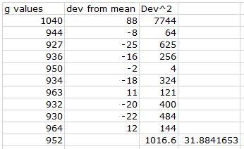
952 in the below graph is the mean g value. The dev from mean column is a formula that subtracts the g value from the mean and puts the result into the dev from mean column. Then, to make all the data positive, the data is squared and entered into the Dev^2 column. The average of the this column is 1016.6. The square-root of this result is the standard deviation value (See Fig. 8) of 31.884 (See Fig. 9)

Fig. 9 Excel data table displaying entire class's g values and the
standard deviation value for all our data.

Conclusion:

This standard deviation tells us how spread out all of our data is. One standard deviation was 31.884. According to theory, 68% of the measured values should be within one standard deviation from the mean, while 95% of data falls within two standard deviations from the mean.

In review, we measured the acceleration of a free-falling object by putting together graphs of position vs time and velocity vs time. In both of these cases, the acceleration given was the amount of gravity acting on the object. We then collected all the class results and put together a table to determine what one standard deviation from the mean value would be. We used this to determine if our data was as precise (spread-out) as is customary, and yes, our data was in line with theory. 

The pattern among all g values was the same, they were all lower than the accepted value of gravity. As discussed above, the reason that these values are lower are due to systematic errors in the equipment, friction in the falling of the object, and air resistance. 

If these errors and assumptions were corrected, I am confident that the values of g would be much closer to 981 cm/s^2.