Lab 13 - April 23, 2015 - Magnetic Potential Energy Lab

Lab 13:
April 23, 2015
Brandon Elder

Magnetic Potential Energy Lab

Purpose:

The purpose of this lab is to verify that the conservation of energy applies to this system of an air track glider and to determine an equation to represent the magnetic potential energy in the system, since this is not easily definable.

Background Info and Set-Up:

Assemble the apparatus as shown in Fig. 1. The apparatus consists of an air track with air hose and a glider that rests on the rack. The glider has a magnet at the end and also a magnet at the end of one side of the air track. The magnets have the same polar ends pointing toward each other so that they do not attract each other, they will push each other away when they get close. Energy will transfer into these magnets and this will become the magnetic potential energy. This is part of what we will be measuring in this system, along with the kinetic energy, to determine that the energy is conserved. We will be measuring this by placing a glider on an airtrack and turning the air on to force the glider as close to the other magnet as possible. The air will be cut off and then the distance they are away from each other will be measured.

Fig. 1 The apparatus with the air glider on the
track and the magnets at both ends.

Fig. 1a The freebody diagram
shows that the F equals mgsin(theta).

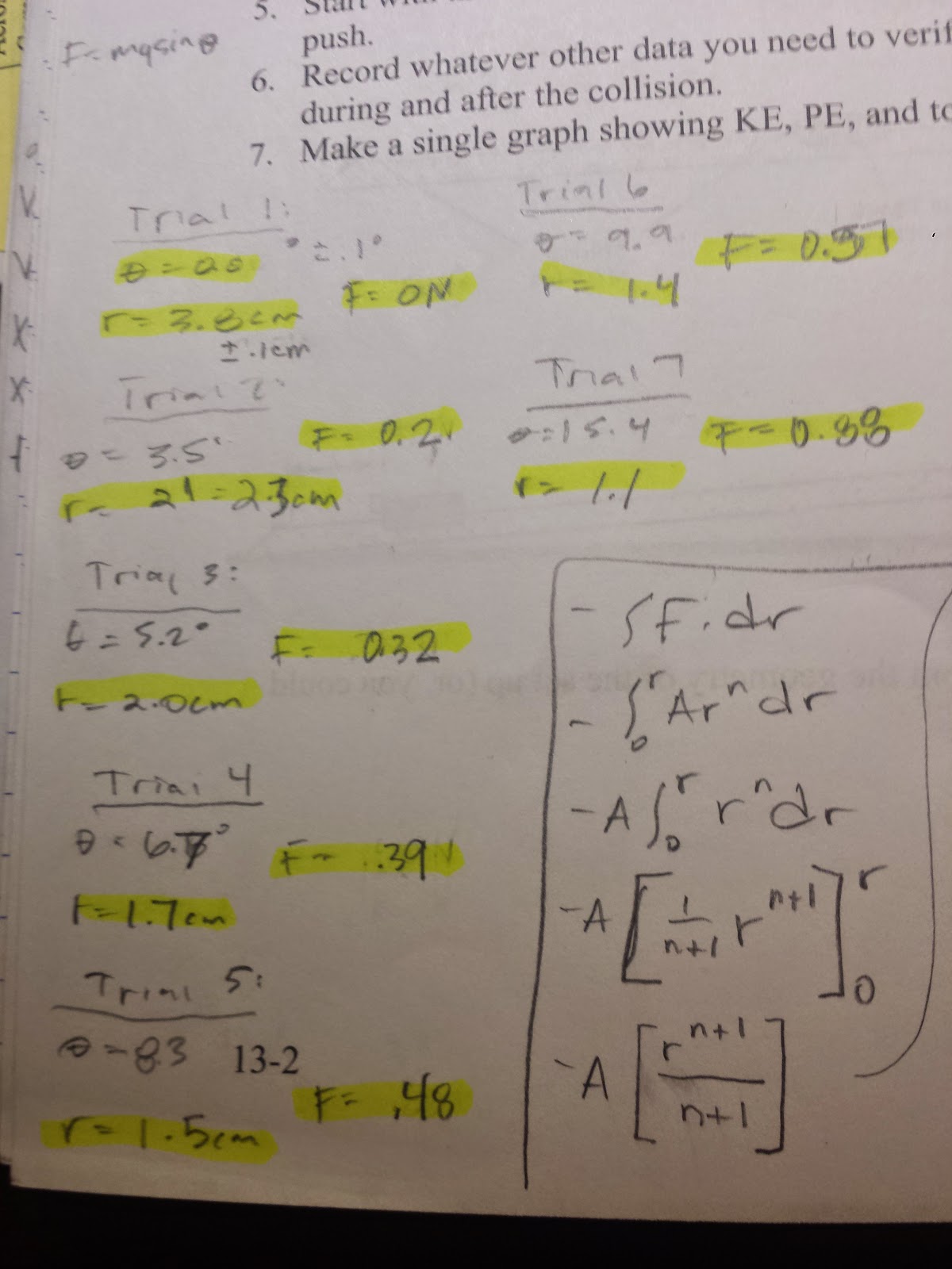Fig. 1b The data used for theta and r
to plug into Logger Pro.

The first step is to level the track. Next, tilt the track at various angles to measure the distance that the two magnets are away from each other, the separation distance r. This data will be recorded along with the magnetic force F. The separation distance and the force will be plotted and then a best fit line will be applied to determine the relationship and the slope. We can safely assume that this will be a power function therefore giving us some sort of power equation F=Ar^n. A and n will be taken from the best fit graph (see Fig. 2). F can be determined by drawing a free body diagram (see Fig. 1a). The velocity will be fixed as the cart approaches the magnet on the end of the track and it will eventually stop moving as it gets as close to possible to the magnet that the current angle will allow for. The kinetic energy of the cart is then converted into the magnetic field between the two magnets and is the magnetic potential energy. As the car is pushed back away from the magnets it is converted back into the potential energy in the air gliders. To the side is the data (see Fig. 1b) that was used and plugged into LoggerPro to calculate the graph from Fig. 2. 

Fig. 2 The best fit line of the graph of the separation distance and the Force. This line gives us the values for A and n.

Now we have an equation for the force between the magnets as a function of their separation, F(r). Integrating this will give us an equation for the magnetic potential energy, which we will write as U(r) (see Fig. 3).

Fig. 3 The integral of F(r) gives us an expression
for the magnetic potential energy U(r).

Fig. 4 The graph showing that the energy is conserved. The top line is the graph of the total energies, the kinetic plus the magnetic. The second line under the peak of the total energy line represents the magnetic potential energy. The bottom line is the that represents the kinetic energy in the glider. It makes sense that at the point where the glider can no longer get any closer to the other magnet, the kinetic energy is transferred into the magnetic potential energy and this is where the middle of the graphs are, the spike and drop.

Uncertainties:

There were many sources of error in our data and alot of this is evident in the graph. Many uncertainties were present, in the measurements (+/- .1 cm), in Logger Pro when it gave us the best fit graph of F(r), the device used to measure theta was accurate to +/- 0.1 degrees. 

Conclusion:

We wanted to show that the conservation of energy is true for our system. We had to determine a function that we could integrate to get the magnetic potential energy as a function of how close the magnets got to each other. With that function, U(r), we can then verify that our original purpose was true, which was that the energy is conserved. According to our final graph, this lab shows us that we are correct (see Fig. 4).