Lab 2 - March 3, 2015 - Free Fall Lab

Lab 2: Free Fall Lab

Brandon Elder

March, 5, 2015

Calculation of Gravity using Excel to Analyze Position and Velocity Data

Fig. 1 The l.5 meter column.

Purpose: The purpose of this free fall lab is to analyze the motion of a free falling body as it drops a known distance and then to record distance-time and velocity-time graphs in order to determine the acceleration (gravity) of the object, which should be 9.8 m/s^2.

Setting Up the Experiment:

The apparatus was set up for us in class already, it is a sturdy column that drops an object 1.5 meters (See Fig. 1). The free-fall body is held at the top by an electromagnet, and when released drops straight down. There is a spark generated that marks the location of the free-fall body every 1/60th of a second on a piece of paper hanging behind the object.

The drop of the object was performed in class by the professor. Each team was then given a length of paper that had the measurements from the spark generator. Each measurement was a dot that corresponded to the position of the falling mass every 1/60th of a second.

Procedure:

Fig. 3 Taped down paper

from free fall apparatus with

dots marking location of object.

The distance was measured in 

centimeters.

Step 1: Each team took the length of paper and taped it down on the desk (See Fig. 2). From there we measured the distance from the start to each dot in centimeters (See Fig. 3). We recorded the measurements for the first 15 or so measurements. All of our recordings were written down so we could transfer them to Excel next.

Fig. 4 Excel columns with
time and distance inputted
and calculated.

Fig. 2 The entire strip taped down.

Step 2: Open up a new Excel document and start inputting the data. The inputted data should look like the following table with the appropriate column headings added (See Fig. 4). The time cells (column A) will have a formula inputted. The first entry (A2) will be 0. The next row (A3) will be the formula: "=A2+1/60". Copy this formula down for as many rows as you have recorded distances. For our group, this was a total of 16 measurements. Column B is the Distance column and will not have a formula. The distance in centimeters will need to be inputted for all measurements (shown below).

Step 3: Collecting the Data: The next step is to set up Excel so that we can eventually plot the data on a graph to observe the graphs of position-time and velocity-time. As seen in Fig X, label the data columns respectively. There will be a formula inputted for the remaining columns as was done for column A. The formulas are summarized below. Column C represents the change in position between two measurements. Column D represents the mid-interval time, or the time every 1/120th of a second. Column E is the speed at the mid-interval times. (Fig. 5) below has the data that we collected.

Column B: Enter: "=A2+1/60" - Fill this formula down into all remaining rows in column B.
Column C: Enter: "=(B3-B2)" - Then fill this cell down through the end of your rows.
Column D: Enter: "=A2+1/120" - Fill down through remaining rows.
Column E: Enter: "=C2/(1/60)" - Fill down all remaining rows.

Fig. 5 Entire Excel data table with all formulas inputted into each column.

Step 4: Graphing your Data: The first graph to put together, using Excel, is the velocity vs time graph. This graph will allow us to calculate a best fit line that will go through the average of the data (See Fig.6). The slope of this line will be the acceleration, which should be a figure close to gravity, 9.8m/s^2 or 980 cm/s^2.

Fig. 6 Chart of  Mid-Interval Time (sec) vs. Mid-Interval
Speed (cm/s). The slope given is our experimental value
for gravity.

In this case, you can see that the slope of the line was 934.71 cm/s^2 (See Fig. 6) which represents the gravity in our experiment. In the graph of position vs time (See Fig. 7), the gravity is half of this number. So, once doubled, it becomes the gravity expression.

Fig. 7 Chart of Position (cm) vs. Time (sec) with best fit line.
The equation of the line is displayed and is our value for
gravity (acceleration) in our experiment.

Step 5: Analyzing the Data: The graphs of mid-interval time as well as the graphs of the regular time interval have the same acceleration. The experimental value of our acceleration, or gravity, is lower than the expected value of gravity, which is 981 cm/s^2. There are multiple reasons why these numbers that we come up with are smaller. Our experiment was not the most accurate experiment to test gravity. For example, there was no factor for air resistance in the experiment. There was also no factor to counter the friction force that is applied on the free falling mass. Lastly, there are some systematic errors introduced into the experiment from the column set up, such as calibration of the equipment.

Determining the Relative Difference:
Regardless of the above errors, we must come up with a way to estimate these errors and to estimate how big these uncertainties will be. One way of estimating these errors is by evaluating the relative difference. This can be done by performing the following calculation:

[(Experimental Value - Accepted Value) / Accepted Vale ] * 100% = Relative Difference %

In the above experiment, our value was: 

[(934.71 - 981) / 981] * 100 = 4.72%

Standard Deviations:

Lastly, we combined all the class data onto one spreadsheet in order to calculate the standard deviations of all our data. These calculations will help determine the accuracy of our returns and to see how reasonably close our experiment's results were to each other. We took the standard deviation of the mean. We collected all our g values that we took off of the graphs. We calculated the standard deviation from the mean by subtracting all the deviations from the mean of all the g values.

Fig. 8 Formula used to calculate
standard deviation of the mean.

952 in the below graph is the mean g value. The dev from mean column is a formula that subtracts the g value from the mean and puts the result into the dev from mean column. Then, to make all the data positive, the data is squared and entered into the Dev^2 column. The average of the this column is 1016.6. The square-root of this result is the standard deviation value (See Fig. 8) of 31.884 (See Fig. 9)

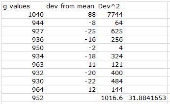Fig. 9 Excel data table displaying entire class's g values and the
standard deviation value for all our data.

Conclusion:

This standard deviation tells us how spread out all of our data is. One standard deviation was 31.884. According to theory, 68% of the measured values should be within one standard deviation from the mean, while 95% of data falls within two standard deviations from the mean.

In review, we measured the acceleration of a free-falling object by putting together graphs of position vs time and velocity vs time. In both of these cases, the acceleration given was the amount of gravity acting on the object. We then collected all the class results and put together a table to determine what one standard deviation from the mean value would be. We used this to determine if our data was as precise (spread-out) as is customary, and yes, our data was in line with theory. 

The pattern among all g values was the same, they were all lower than the accepted value of gravity. As discussed above, the reason that these values are lower are due to systematic errors in the equipment, friction in the falling of the object, and air resistance. 

If these errors and assumptions were corrected, I am confident that the values of g would be much closer to 981 cm/s^2.